On the Probability Flow ODE of Langevin Dynamics

• 1. Introduction
• 2. Langevin dynamics and its probability flow ODE
  • 2.1. Probability flow ODEs
  • 2.2. Estimating the vector field via the binary classification
• 3. Modifying the code of GANs

1. Introduction

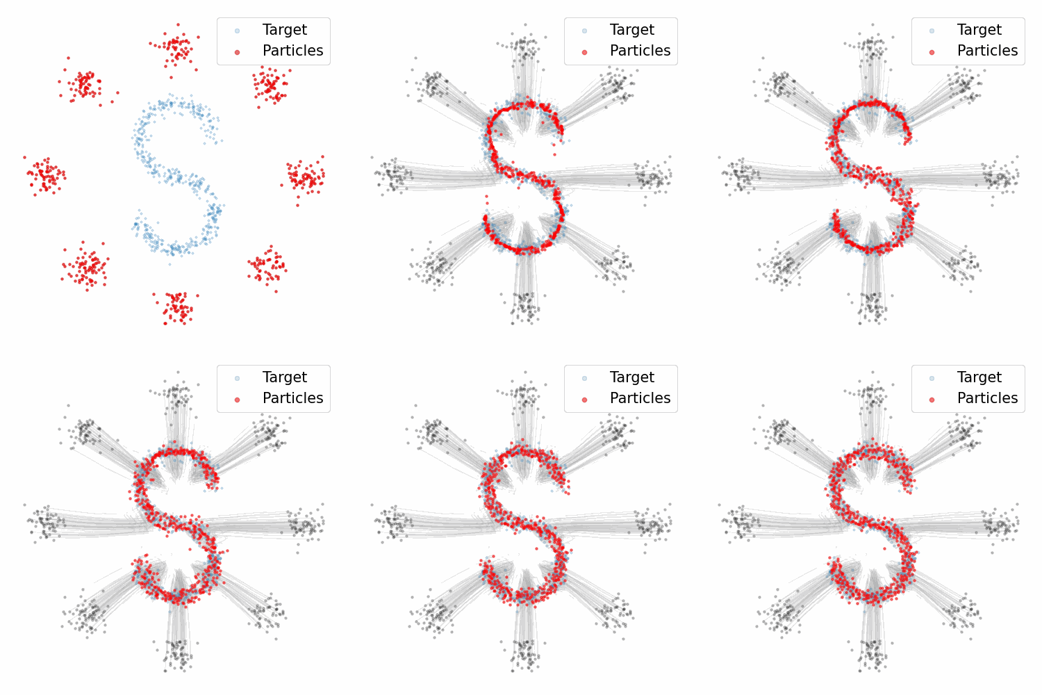
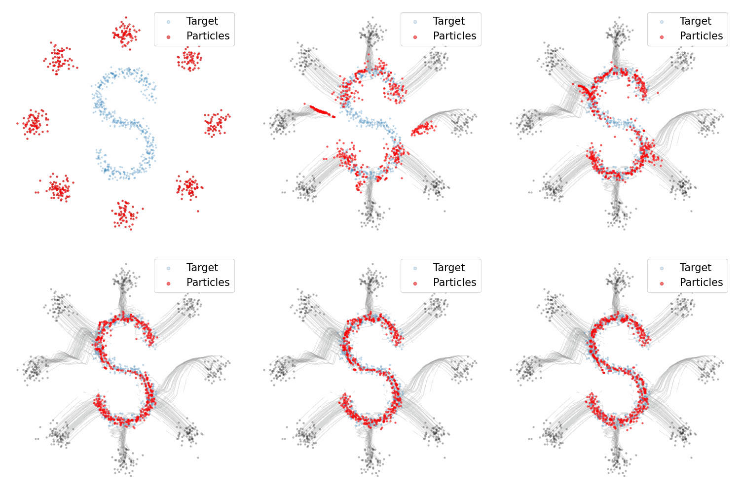
This post provides a simple numerical approach using PyTorch to simulate the probability flow ordinary differential equation (ODE) of Langevin dynamics. The implementation is super simple, one just needs to slightly modify a code of Generative Adversarial Nets. Such an implementation can be understood as ‘‘non-parametric GANs’’, which is an alternative view via the probability flow ODE, more details can be found in my paper ‘‘MonoFlow: Rethinking Divergence GANs via the Perspective of Wasserstein Gradient Flows’’. Briefly speaking, we can remove the generator in GANs and simulate a probability flow ODE similar to diffusion models.

The above demo uses a modified version of Radford Neal’s funnel distribution. The funnel distribution is known to be difficult to sample from due to its irregular geometric properties. Langevin dynamics utilizes the log density information to explore the distribution but its particles fail to reach the bottom area of the funnel. The probability flow ODE succeeds in this task as it does not rely on the density function but on samples drawn from the target distribution.

All jupyter notebooks can also be found on .

Additionally, the paper ‘‘Unifying GANs and Score-Based Diffusion as Generative Particle Models’’ and ‘‘GANs Settle Scores!’’ provide explorations of non parametric versions of Integral Probability Metric GANs.

2. Langevin dynamics and its probability flow ODE

Langevin dynamics follows a stochastic differential equation (SDE) to describe the motion of a particle \(\mathbf{x}_t \in \mathbb{R}^n\), \begin{aligned} \mathrm{d} \mathbf{x}_t = \nabla_\mathbf{x} \log p(\mathbf{x}_t)\mathrm{d}t + \sqrt{2} \mathrm{d}\mathbf{w}_t, \end{aligned} where \(\mathbf{w}_t\) represents the Brownian motion. Using the Itô integration, we can obtain the Fokker-Placnk equation describing the marginal laws of the dynamics over time, \begin{aligned} \frac{\partial q_t(\mathbf{x})}{\partial t} = \text{div}\Big[ q_t(\mathbf{x})\big(\nabla_\mathbf{x} \log q_t(\mathbf{x}) - \nabla_\mathbf{x} \log p(\mathbf{x}) \big) \Big], \end{aligned} where \(\text{div}\) is the divergence operator in vector calculus.

If the target distribution decays at infinity \(\lim_{\mathbf{x} \to \infty} p(\mathbf{x})= 0\), e.g., the Boltzmann distribution \(p(\mathbf{x}) \propto \exp\big(-V(\mathbf{x})\big)\), the equilibrium (steady state) of the dynamics is achieved if and only if \(q_t=p\) such that the infinitesimal change of the marginal is \(\frac{\partial q_t}{\partial t}=0\). Evolving a particle from the initialization \(\mathbf{x}_0 \sim q_0(\mathbf{x})\), its marginal \(q_t(\mathbf{x})\) will eventually converge (weakly) to the stationary distribution \(p(\mathbf{x})\). However, establishing the convergence rate within finite-time can be challenging; additional conditions for the target distribution must be met to guarantee convergence. For example, if \(p(\mathbf{x})\) satisfies the log-Sobolev inequality, then the marginal \(q_t(\mathbf{x})\) will converge to \(p(\mathbf{x})\) exponentially fast in terms of the Kullback-Leibler divergence. Nevertheless, we shall be able to expect that Langevin dynamics can at least find some local modes in practice.

In order to numerically simulate Langevin dynamics, we can use the Euler-Maruyama method to discretize the SDE, this gives the well-known unadjusted Langevin algorithm (ULA), \begin{aligned} \mathbf{x}_{i+1} \leftarrow \mathbf{x}_{i} + \epsilon \nabla_{\mathbf{x}} \log p(\mathbf{x}_i) + \sqrt{2\epsilon} \mathcal{N}(0, I), \quad i=0, 1, 2\cdots \end{aligned} Iteratively running ULA, we can gradually transport samples from \(q_0(\mathbf{x})\) to \(p(\mathbf{x})\) as shown in the previous demo to sample from the funnel distribution. ULA is widely used in large-scale machine learning. For example, it can be applied in the training of Bayesian neural networks and energy-based models, and it also serves as the sampling scheme for the earliest version of score-based diffusion models (Song and Ermon, 2019).

2.1. Probability flow ODEs

There are several approaches to derive the probability flow ODE of Langevin dynamics. The most accessible one is using the result from score-based diffusion models. In score-based diffusion models, it is shown that each SDE has an associated probability flow ODE sharing the same marginal \(q_t\) (also see the Eq. (13) in Song et. al., 2021). Simply using this result, we can convert the Langevin SDE to the associated ODE, \begin{aligned} \mathrm{d} \mathbf{x}_t = \Big [\nabla_\mathbf{x} \log p(\mathbf{x}_t)- \nabla_\mathbf{x} \log q_t(\mathbf{x}_t)\Big]\mathrm{d}t. \end{aligned} The marginal laws of the probability flow ODE also follow the same Fokker-Planck equation. The probability flow ODE differs from Langevin dynamics only in the nature of particle evolution: the former is deterministic, while the latter is stochastic. Similarly, using the Euler method to discretize the ODE gives \begin{align} \mathbf{x}_{i+1} \leftarrow \mathbf{x}_{i} + \epsilon \big[\nabla_{\mathbf{x}} \log {p(\mathbf{x}_i)}- \nabla_{\mathbf{x}} \log {q_{i}({\mathbf{x}_i})}\big], \quad i=0, 1, 2\cdots \end{align} It is worth noting the vector field of the probability flow ODE is the gradient of the log density ratio \(\log \big[p(\mathbf{x}_i) / q_{i}({\mathbf{x}_i})\big]\). If we have access to the log density ratio, we can use the Euler method to simulate the ODE. Next, we will discuss a method to obtain the log density ratio, analogous to training the discriminator in GANs.

2.2. Estimating the vector field via the binary classification

Recall that in GANs, we train a discriminator to solve the following binary classification problem, \begin{aligned} \max_D \qquad \mathbb{E}_{p} \big[\log D(\mathbf{x})\big]+ \mathbb{E}_{q_i} \big[\log (1-D(\mathbf{x}))\big]. \end{aligned} The optimal discriminator is given by (see Proposition 1 in Goodfellow et. al. 2014), \begin{aligned} D^{*}(\mathbf{x}) = \frac{p(\mathbf{x})}{p(\mathbf{x}) + q_i(\mathbf{x})} \end{aligned} Since the last layer of the discriminator \(D^{*}(\mathbf{x})\) is activated by the Sigmoid function \(\sigma(\cdot)\), inversing the Sigmoid activation gives the log density ratio, \begin{aligned} \sigma^{-1}\big(D^{*}(\mathbf{x})\big) =\log \frac{p(\mathbf{x})}{q_{i}({\mathbf{x}})}, \end{aligned} \(\sigma^{-1}\big(D^{*}(\mathbf{x})\big)\) is called the logit output of a binary classifier.

This gives us a strategy for sampling via the probability flow ODE with bi-level optimization which is similar to training GANs,

• Training the discriminator with a few steps of gradient update using samples from \(q_i\) and \(p\).
• Computing the gradient of the logit output and updating particles using Eq. (1).

In the conventional GAN theory, training the discriminator was designed to estimate the Jensen-Shannon divergence (JSD), however, the smoothness between the estimated JSD and the generator’s distribution does not exist in practice because the divergence is reconstructed using samples. One can imagine that the Monte Carlo evluation of the binary cross entropy involves a discrete step–sampling. This is the major reason causing the inconsistency between the GAN theory and its practical algorithms, e.g., the non-saturated tricks. The essential information we obtained in training the discriminator is not the JSD, but is the density ratio function which indicates the vector fields.

3. Modifying the code of GANs

• The first step is to remove the generator G(z), instead we initialize \(512\) particles xs and put them into the SGD optimizer corresponding to the Euler discretization of the ODE. One can also use optim.Adam([xs], lr = 0.001) to incorporate the momentum of gradients. Note that we use the loss function criterion nn.BCEWithLogitsLoss(), this criterion directly works with the logit output of a binary classifier where D_logit is a MLP in this example.

data_dim = 2
# loss
criterion = nn.BCEWithLogitsLoss()

# build network
D_logit = Discriminator().to(device)
-G = Generator().to(device)
+xs = make_8gaussians(n_samples=512).to(device)
+xs.requires_grad = True

# optimizer
D_optimizer = optim.Adam(D_logit.parameters(), lr = 0.001)
-G_optimizer = optim.Adam(G.parameters(), lr = 0.001)
+G_optimizer = optim.SGD([xs], lr = 0.001)

• The next step is to modify the training procedure of GANs. There is no difference on training the discriminator, we just replace fake samples with a minibatch of xs and use a single step gradient descent to train the discriminator. The G_loss is now changed to -torch.sum(D_logit(xs)) with the purpose of computing the per particle gradient. This is because there is no explicit way to perform batch gradient operation by backpropagating the loss in PyTorch, we can instead sum all per particle forward pass together to generate a scalar and backpropagating this scalar would give each particle its own gradient. An alternative is to use torch.autograd class but it could be more complicated.

#==============Train the discriminator===============#
D_optimizer.zero_grad()
# eval real loss on p
x_real, y_real = x.view(-1, data_dim), torch.ones(batch_size, 1).to(device)
real_loss = criterion(D_logit(x_real), y_real)

# eval fake loss on q_i
-z = torch.randn(batch_size, z_dim).to(device)
-x_fake, y_fake = G(z), torch.zeros(batch_size, 1).to(device)
# randomly select some particles to train the discriminator
+idx = np.random.choice(xs.shape[0], batch_size, replace=False)
+x_fake, y_fake = xs[idx], torch.zeros(batch_size, 1).to(device)
fake_loss = criterion(D_logit(x_fake), y_fake)

# gradient backprop & optimize ONLY D's parameters
D_loss = real_loss + fake_loss
D_loss.backward()
D_optimizer.step()

#==============Update particles===============#
G_optimizer.zero_grad()
-z = torch.randn(batch_size, z_dim).to(device)
-x_fake, y_fake = G(z), torch.ones(batch_size, 1).to(device)
-G_loss = criterion(D_logit(x_fake), y_fake) # non-saturate trick
# update all particles
# allow for the batch gradient for each particle
+G_loss = -torch.sum(D_logit(xs))
G_loss.backward()
G_optimizer.step()

So, that’s it! We have deleted 7 lines and added 6 lines. Now we can run the code to simulate the probability flow ODE.

The full code for the S curve is available at .